Wugi's hoom Wugi's DemoComplex
Interactieve
4D visualisaties voor Complexe Functies -
Interactive 4D visuals of Complex Functions  

Guido "Wugi" Wuyts @ Dilbeek, Belgium, Europe, World, Solar System, Milky Way, Local Cluster, ...

@ 3 Taalzaak
@ 2 Denkzaak
@ 1 Smaakzaak
@ 0 Wugi's hoom
Relatieve tijd
QBasics
Font & script
NieuwsDenk
O, redactie
NPN
Readers' Indigest
NewsThink
Mathness
Wugi's Interactive 4D Visuals for
Complex Functions
   (2023)

QBasics :         a QB application site, parent page of:

QBComplex :   'True 4D' visuals of Complex Functions w=f(z),
                           also of other higher-dimensional objects.
                           Parent page of this one.

GOTO Desmos 4D-visuals

GOTO Geogebra 4D-visuals

GOTO Desmos3D visuals   (complex "true curves" page)

GOTO Desmos3D 4D-visuals


Complex Function 4D Visuals in Desmos

Complex Function 4D Visuals in Geogebra

The following visualisations are Desmos files, allowing toying with the parameters and animating the graph.
They are visualisations of complex functions w=f(z), where z=x+iy and w=u+iv are complex variables.
The "Info" entries can be opened with the triangle icons to read information about the topic.
The "Control" entries can be opened with ditto icons, to find slider controls for changing or animating variables.
The "Show" entries can be activated by clicking in the empty circle icons, to visualise the topic items.


Another interactive tool at our disposal is Geogebra.
The great advantage of it is its 3D (x,y,z) graphing capability, with surface texture's coloring and transparency.
Its editor though is very shaky, with arbitrary results when trying to select a piece of text or formula, no control where to put and group your formulas (it groups and orders them by type, not by one's logical objects), jumping to its top position after confirming each edit, accidental delets and saves...
Anyway, it's nice to compare this output with the previous.
And I'm abiding the epoch when mainstream mathwizz software will finally discover this "true 4D" method, and incorporate it in its powerful rendering libraries.

I've grouped all next examples in this 'public book':
https://www.geogebra.org/m/bmuqbufn


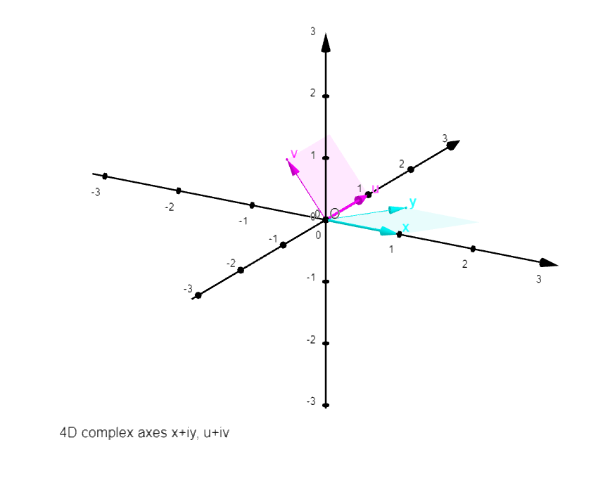
A 4D coordinate system in 2D:

Axes x and u coincide originally with the graph's orthogonal coordinates X and Y, with same units (°). Axes y and v are projected upon the graph's X,Y plane, so that the units of the axis pairs x,y and u,v belong to ellipses which represent projected circles around the origin. These axis projections are described
by three values:
the shorter axis (y or v unit; the greater axis=1: x or u unit): see b and bw;
a tilt angle of the ellips: see d and dw;
a rotation angle of x,y or u,v in their respective ellips: see j and jw.

(°)
The "real plane" (x,u) can be made to coincide with the graph plane X,Y by changing the 4D axes controls to the values:
b=d=j=bw=jw=0, and dw=pi/2 (~1.57)
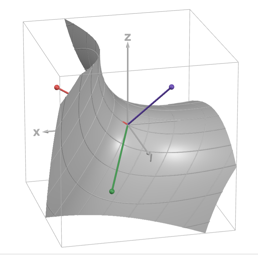
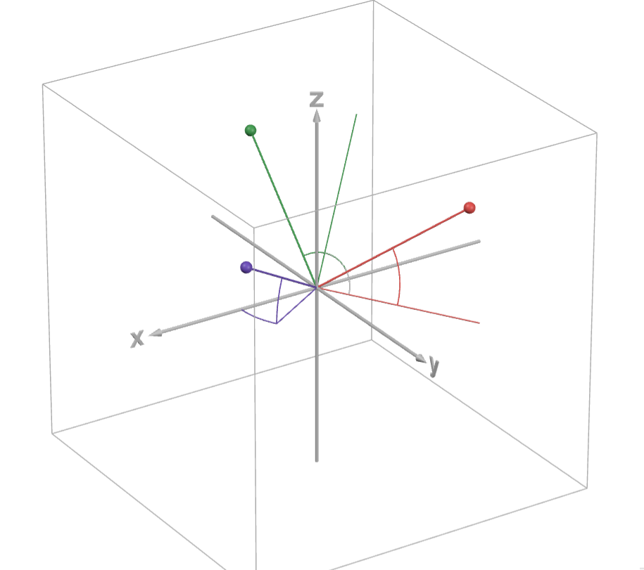

A 4D coordinate system in "3D in 2D":

Axes x and u coincide with the graph's coordinates X and Y, with same units. Axes y and v are projected upon the graph's X,Y,Z space, along unit vectors determined by two angles each:

b_y and b_v = angle of y and v projections in the X,Y plane;
c_y and c_v = angle of y and v with their X,Y projection, along Z dimension.


In the function graphs, controls L and M are for parameter curves.

Some graphs have earlier versions with 3 axes coinciding with the graph's, and a fourth projected upon those.


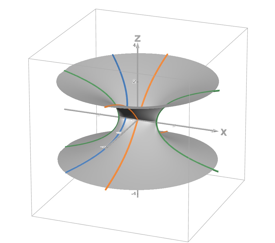
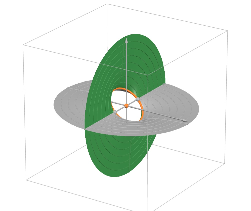
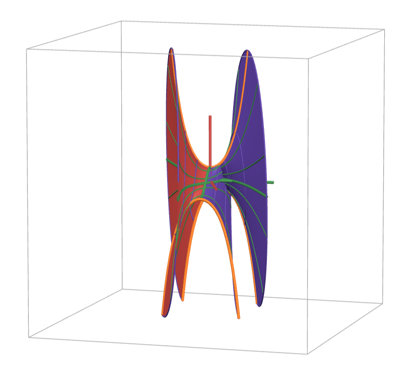
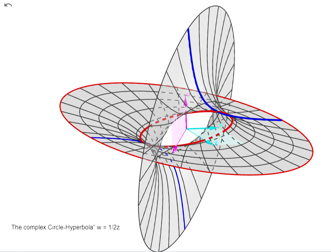
The Circle-Hyperbola:
w = 1 / 2z

 
There are two asymptotes: w=0 (the z plane) and z=0 (the w plane, a pole: w->infinity), see the two "blades" approaching the coordinate planes at infinity.
The red curves are hyperbolas (like the "real" one in the x,u plane). The blue ones are circles (like the central one, with radius 1 and real points (x,u)=(0,+/-1)). That's why I call this function the Circle-Hyperbola!
Circle and hyperbola are curves of the same surface in complex space.
The complex function surfaces
ww+zz=1, ww-zz=1, ww+zz+1=0, w=1/z*sqrt(2)
represent a single surface, in different orientations with "real curves" circle, hyperbola, imaginary circle, and hyperbola respectively.

earlier version:

https://www.geogebra.org/calculator/kkp6d58s
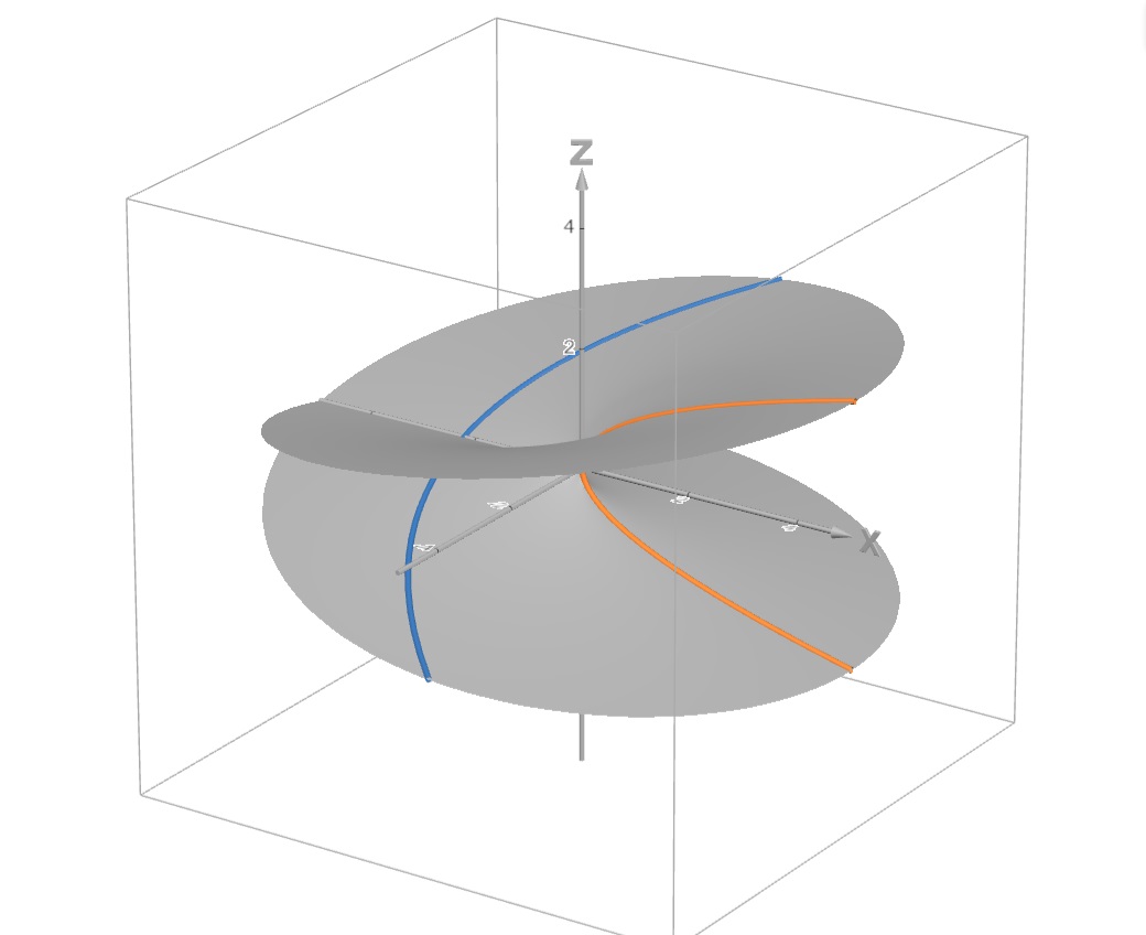
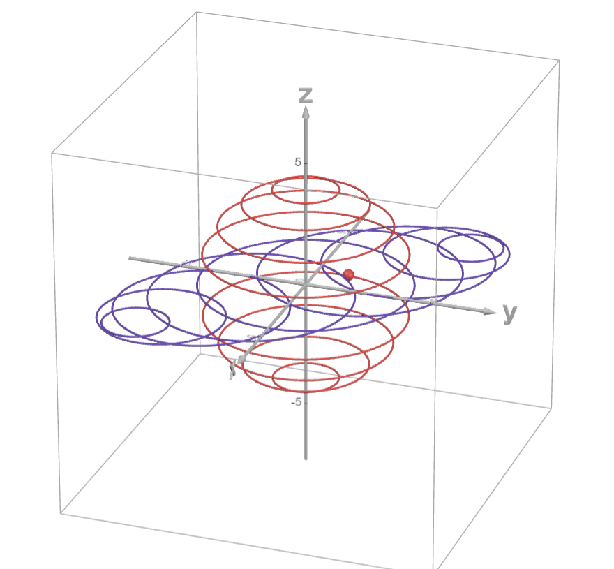
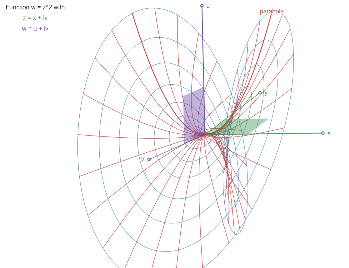
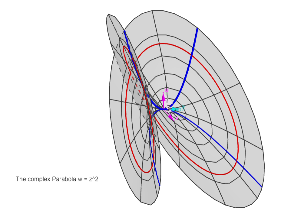


The Parabola:
w = z^2


A "4D paraboloid", with parabolas (in red, like the "real" one in the x,u plane) rotating in complex space, following their z-coordinates rotating in the z=x,y plane.

Earlier version:

https://www.geogebra.org/calculator/bw3xgauv 


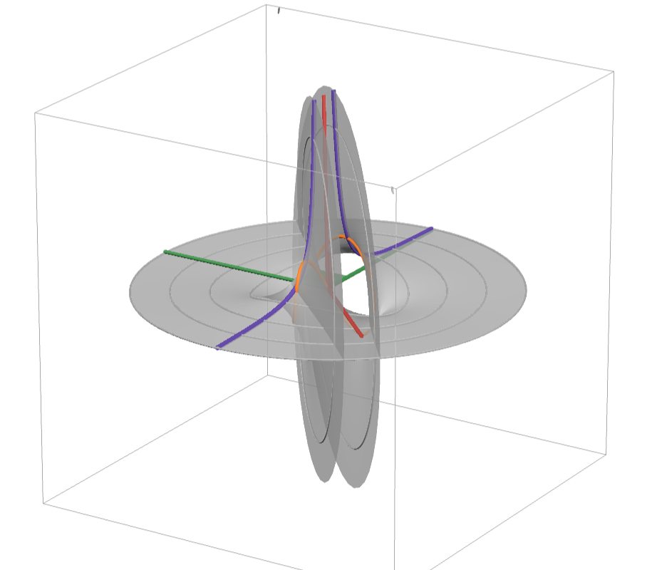
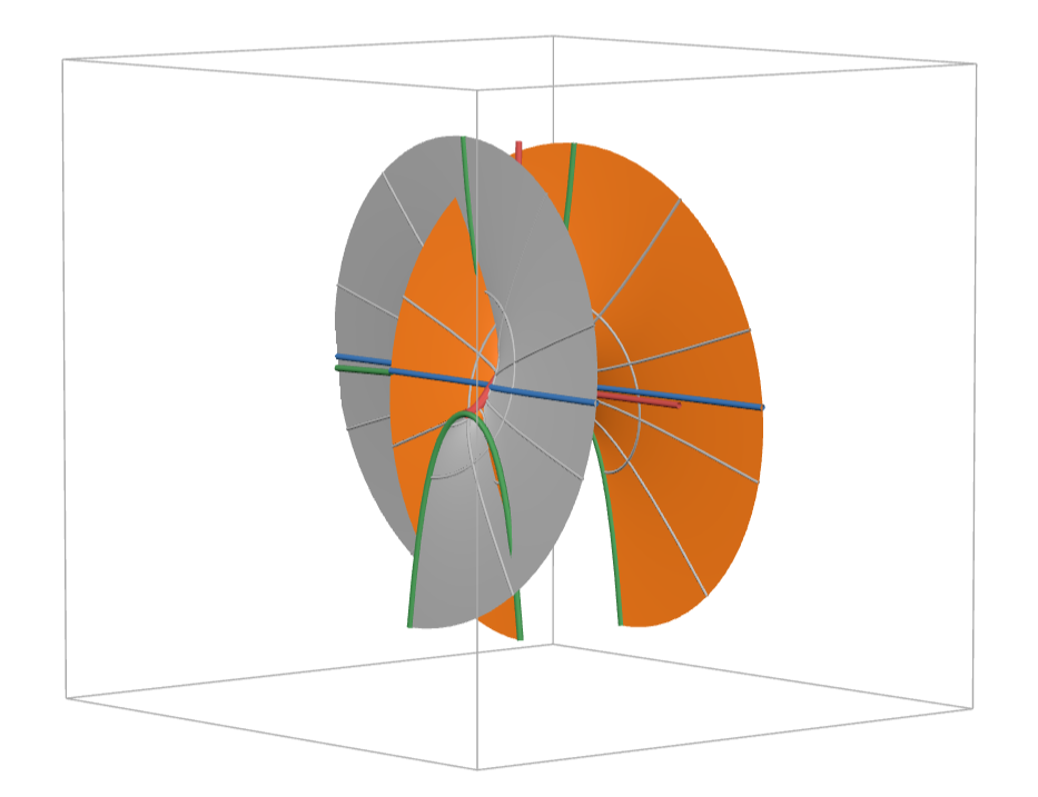
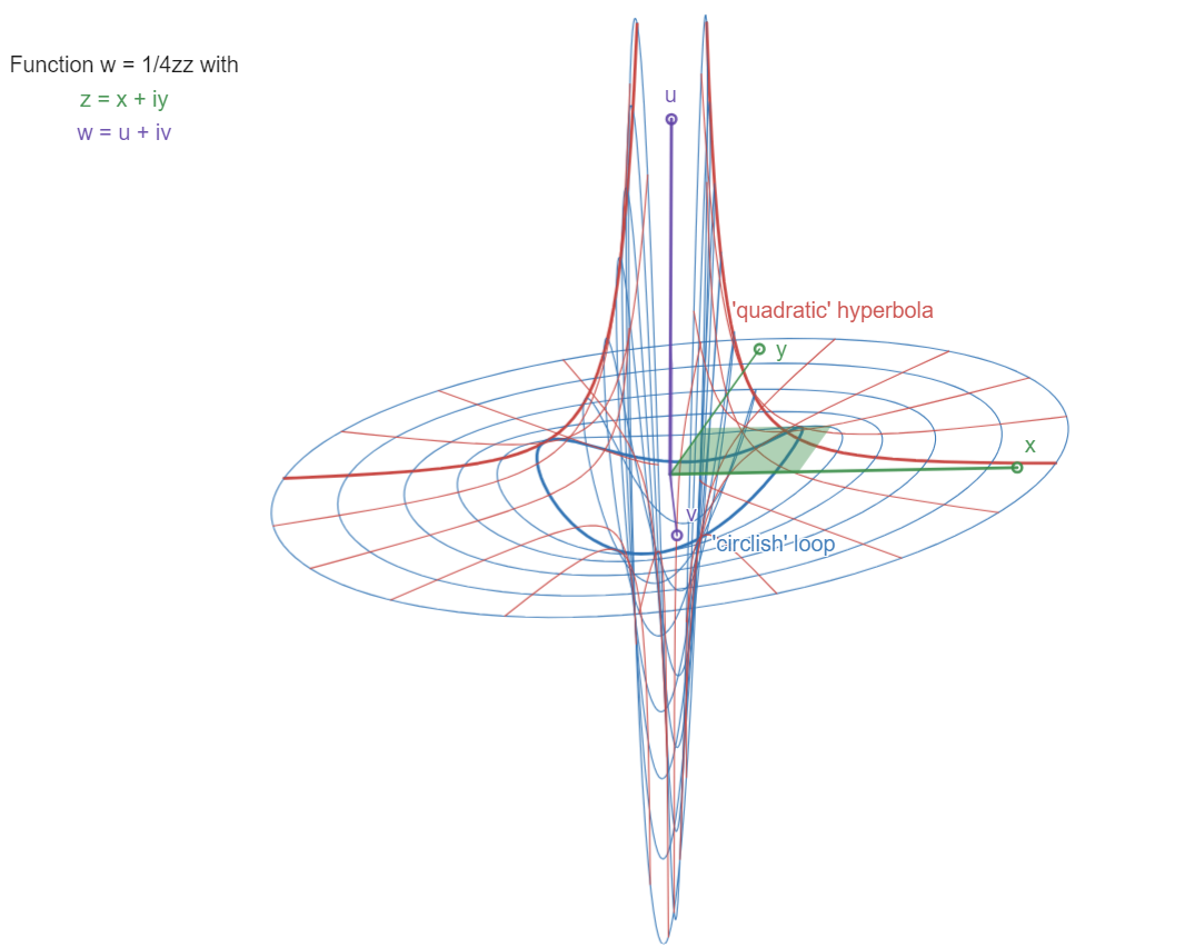
The "quadratic" Hyperbola:
w = 1 / 4z^2

There are two asymptotes: w=0 (the z plane) and z=0 (the w plane, a pole: w->infinity, and yet a double one), see the two "blades" approaching the coordinate planes at infinity, the w-blade double (w rotates twice for one z-rotation). The function is oriented with u,v plane "frontal" so as to separate the double w-blade view.
Compare with the function w=1/2z, the "Circle-Hyperbola" (its double name describing its parameter families). Here we have "circlish" closed loops in blue, and "quadratic hyperbola" twin curves in red.

Earlier version:

https://www.geogebra.org/calculator/kb6sqtf9
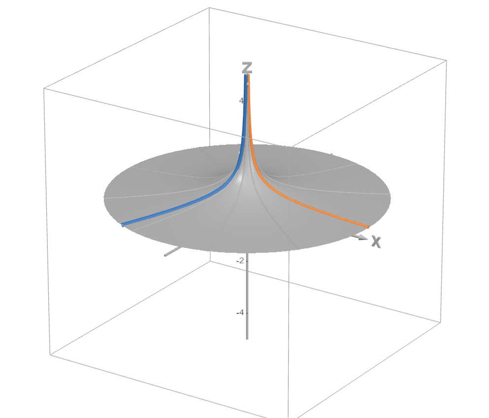
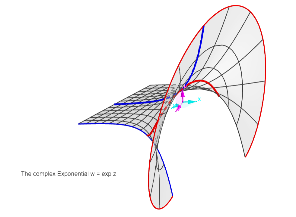


The Exponential:
w = exp z

Periodic function along y=Im(z) axis, period 2pi. One period is shown, from -pi to +pi.
There is one asymptote: w=0 (the z plane), see the "blade" approaching the coordinate plane at infinity to the left.
The red curves are exponentials (like the "real" one in the x,u plane), the blue ones are semi-sinusoids (like the "semicosine" through the origin). That's why the exponential and its reciprocal exp -z taken together will form Sine functions (see graph of the Cosine)! The asymptotes "left" and "right" will disappear, leaving the reciprocal blades "left" and "right", separated by a sine or cosine curve.

Earlier version:

https://www.geogebra.org/calculator/zufs5s44
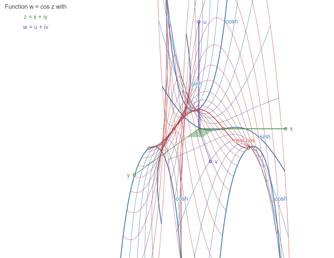
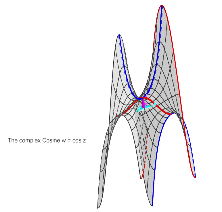


The Cosine:
w = cos z = 0.5*(exp z + exp -z)

Periodic function along x=Re(z) axis, period 2pi. One period is shown, from -pi to +pi.
The asymptotes of the exponential (see graph of that function) and its inverse disappear, leaving two opposite exponential blades.
The red curves are sinusoids, minimised at the real cos curve (in the real plane x,u). The blue ones are hyperbolic cosinoids, with periodic cosh and sinh curves. 


Earlier versions:

https://www.geogebra.org/calculator/r8gxrmpf

https://www.geogebra.org/calculator/w8pmnpfu
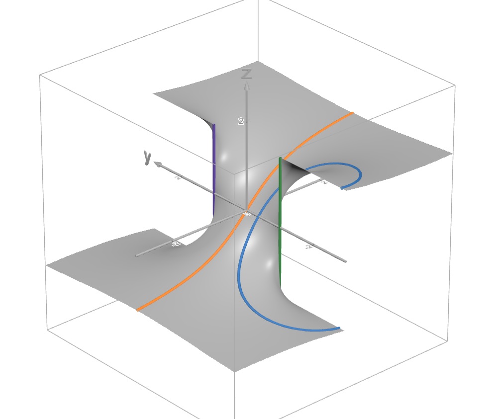
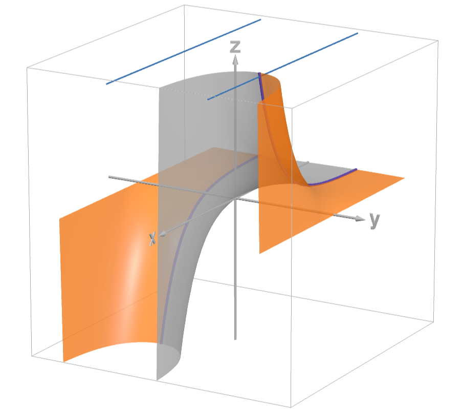
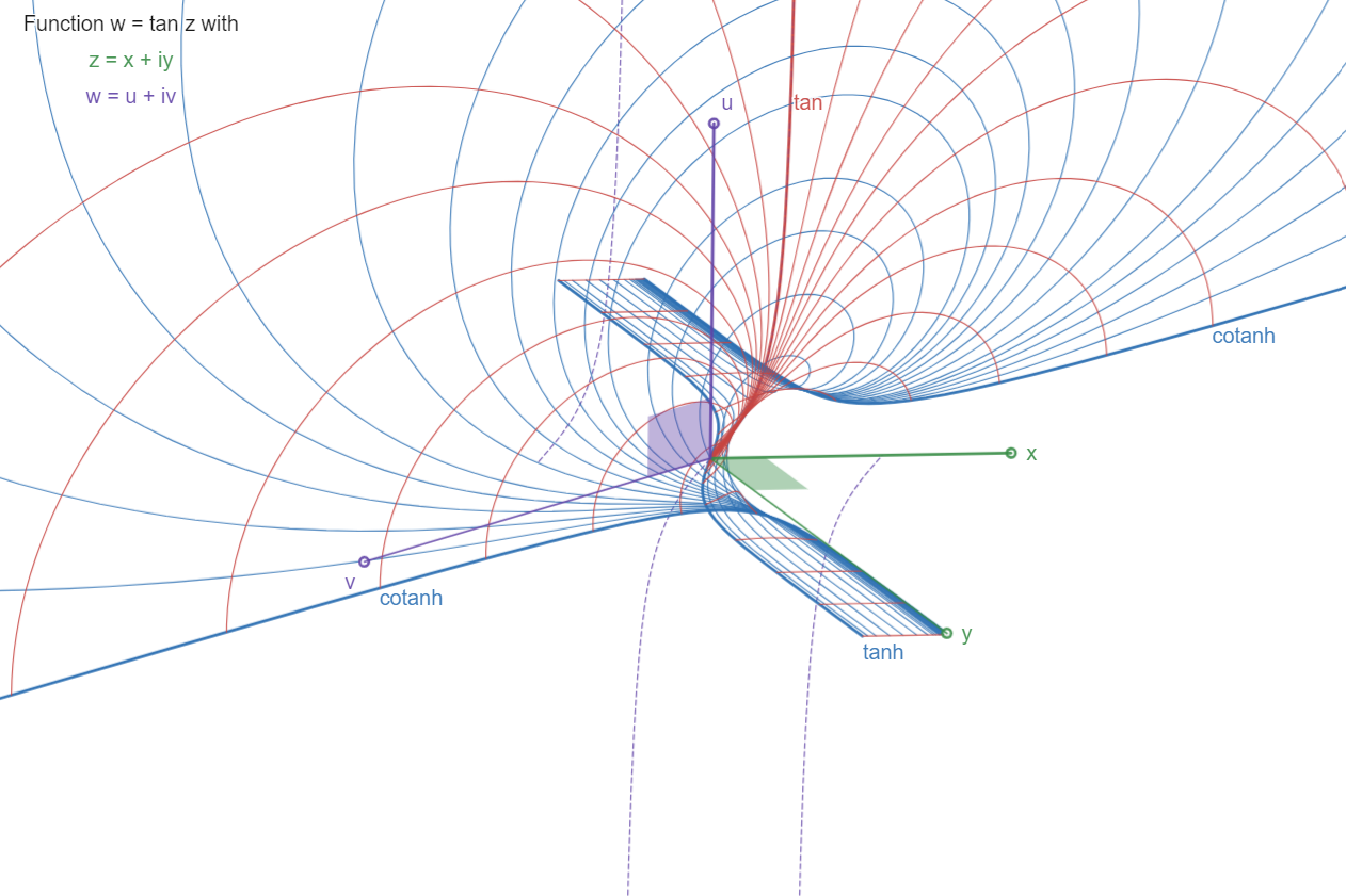


The Tangent:
w = tan z

Periodic function along x=Re(z) axis, period pi. A half period is shown, from x=0 to +pi/2. The hatched curve shows more of the real function u=tan x, in the x,u plane.
The surface approaches asymptote plane x=pi/2 (parallel to the u,v plane) by its "expanding" blade, which contains the real curve
u=tan x,
and is limited by the curves
v=tanh y,  for x=0, in the y,v plane, and 
v=cotanh y,  for x=pi/2, in the parallel plane.
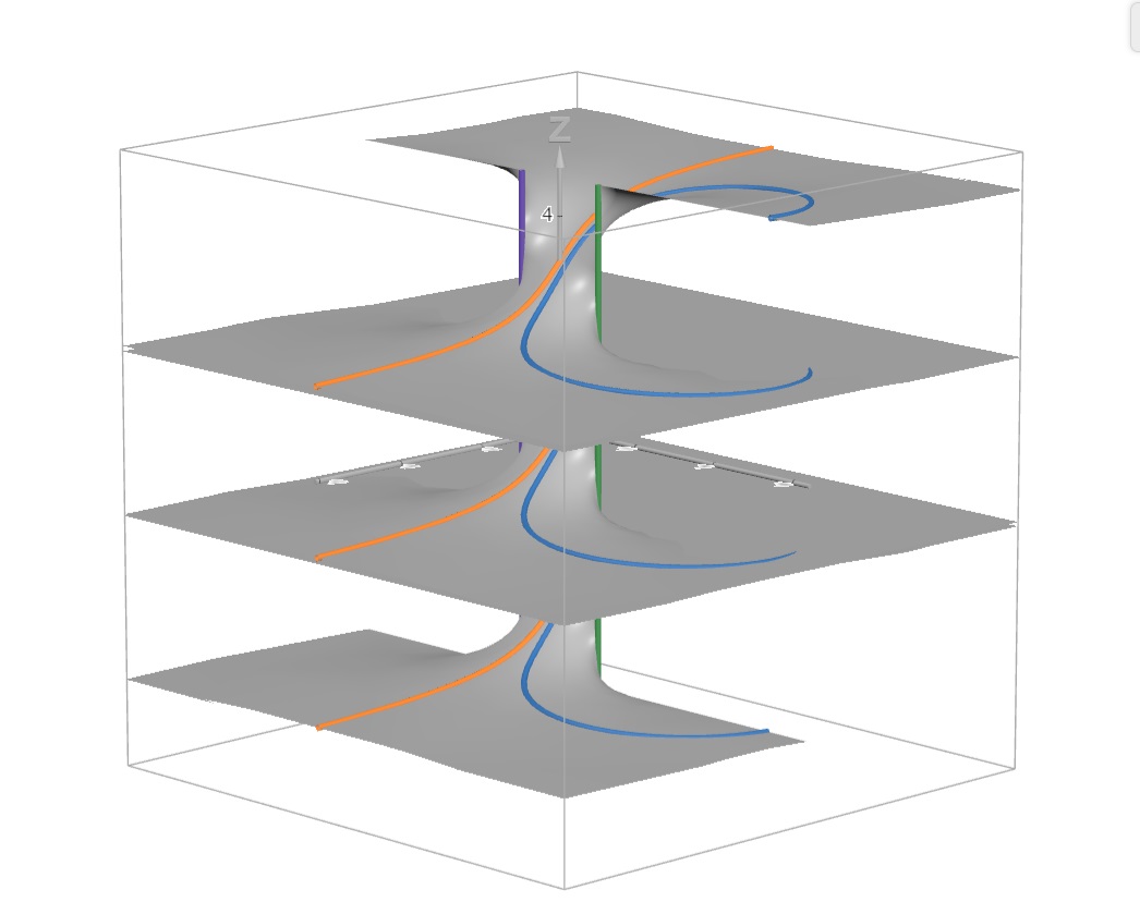
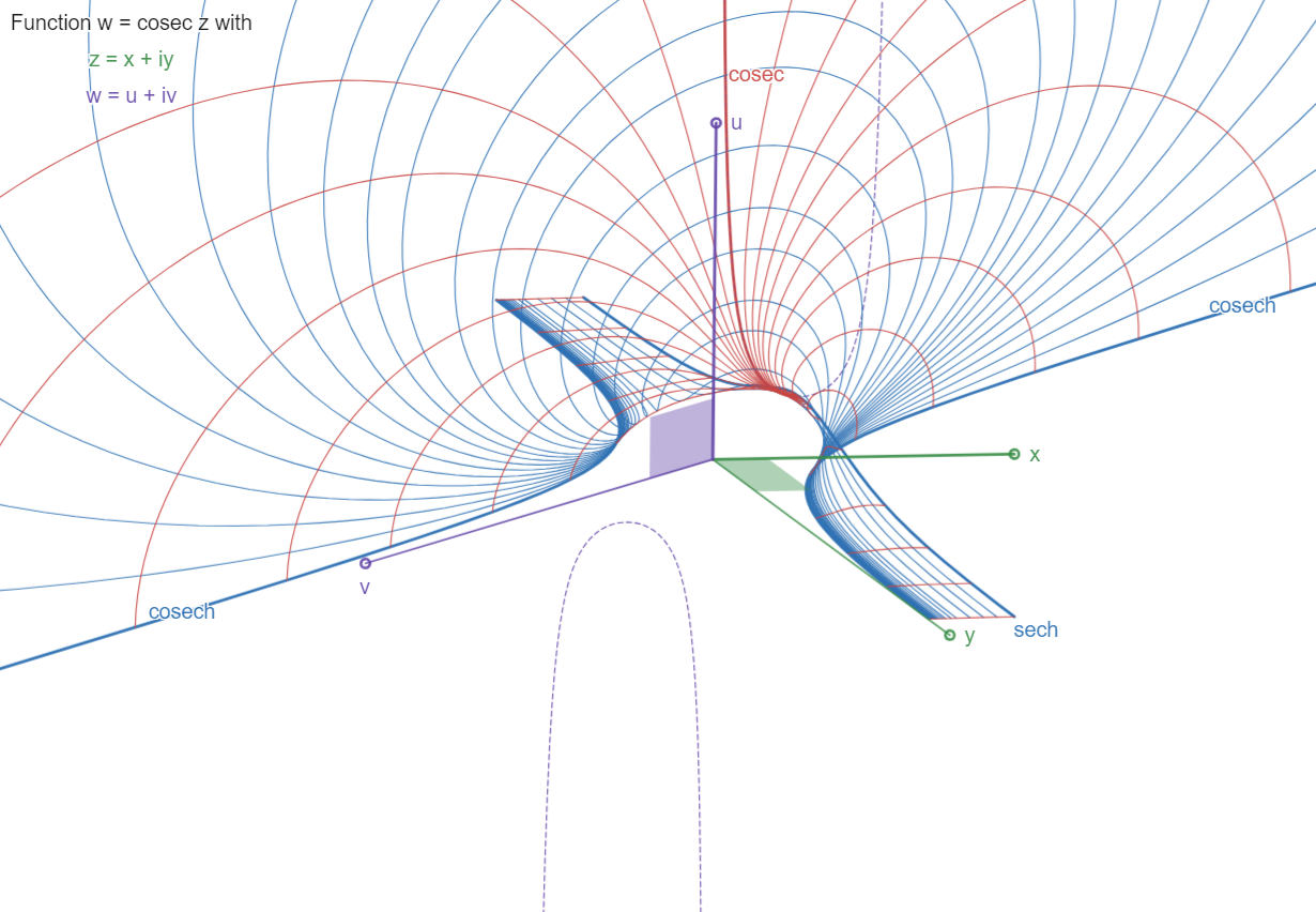


The Cosecant:
w = csc z

Periodic function along x=Re(z) axis, period 2pi. A quarter of a period is shown, from x=0 to pi/2. The hatched curve shows more of the real function u=csc x, in the x,u plane.
 
The surface approaches asymptote plane x=0 (the u,v plane) by its "expanding" blade, which contains
the real curve
u=cosec x
and is limited by the curves
u=sech y, for x=pi/2 parallel to the y,u plane, and
v=cosech y, for x=0 in the y,v plane.


Complex Function Visuals in Desmos 3D :    True curves and their 3D surfaces, of complex functions

Given z=x+iy, w=u+iv, a function w=f(z), and its function surface in 4D space (x,y,u,v).

Keeping x constant results in a curve in 3D space (y,u,v).
Same for y constant, with a curve in (x,u,v) space.
These are
true curves, meaning that they are a geometrically true part of the 4D function surface.

Making x a parameter in the function equation w=f(z), results in a surface
in (y,u,v) space: the x-surface of true curves x=cst.
With y as a parameter, we get another surface, the y-surface of true curves y=cst in (x,u,v) space.

With polar coordinates z=Z e^iζ, we obtain a (Z,u,v) curve, and a ζ-surface of them.

More on
True curves in my Youtube channel, here and here.

The following pictures show the results for some typical functions, with the links to their
Desmos 3D example. Curves shown are with cartesian coordinates, unless polar is mentioned.


Cosine w = cos z
One period shown.
Characteristic curves: cos, cosh, sinh


Cosine w = cos z
One period shown, but sliding between two periods


Sine w = sin z
One period shown.
Char. curves: sin, sinh, cosh


Tangent w = tan z
One period shown.
Char. curves: tan, tanh, coth


Tangent w = tan z
Three periods shown


Cotangent w = cot z
One period shown, but sliding between two periods.
Char. curves: cot, coth, tanh


Exponential w = exp z
One period shown, but sliding between two periods.
Char. curve: exp


Parabola w = zz
'square' view
All curves are flat: parabolas!
Char. curve: real parabola


Parabola w = zz
Same surface as previous, but 'rounded' view


Parabola w = zz
Polar curves
Char. curve: real parabola (two halves)


Square root w = z^(1/2)
Polar curves
Comparison with quadratic w = zz, parabola


Hyperbola-Circle  w = 1/z
Char. curve: real hyperbola


Circle-Hyperbola  w = 1/z
Polar curves
Char. curves: real hyperbola and minimal circle
also this link with newer version


"Quadratic hyperbola"  w = 1/zz
Char. curve: real curve u = 1/xx


"Quadratic hyperbola"  w = 1/zz
Polar curves
Char. real curve, two halves

More true curves yet!

The conventional 3D graphs of complex functions comprise Re(w) and Im(w), in other words the graphs in (x,y,u) and (x,y,v) space.

Conventional curves on these graphs are x=cst and y=cst (x or y kept constant). These are generally not true curves!
For a curve in (x,y,u) to be true, we'll need to keep v constant. Ditto in (x,y,v) where u must remain constant. So then, u=cst and v=cst are conditions to obtain true curves in the corresponding graphs, Im(w) and Re(w).


Exponential  w = exp z


Cosine w = cos z


Complex function 4D visuals in Desmos 3D!

Now also
4D in Desmos 3D!

The full 4D-graphs of complex functions w = f(z).

The z-plane (x,y) lies in Desmos's (X,Y) plane. It may rotate° within itself, a being the angle between X- and x-axis.

The w-plane (u,v) is perpendicular, so it contains Desmos's Z-axis. It makes an orientation angle b with the X-axis.
It may rotate° within itself, c being the angle between the (X,Y) plane and the u-axis.

° Notice that in 4D-space a double rotation is allowed for solid bodies, within two planes that are doubly-perpendicular to each other, such as our z- and w-planes!


Exponential  w = exp z


Cosine w = cos z


w = exp z and w = exp-z, two 'halves' of the cos z graph!


w = 1/z, a circle-hyperbola


w = 1/z^2, a 'quadratic' hyperbola


w = cos z and w = cosh z
same surfaces, other orientation (here cosh)


MORPH w(z) between  cos z  and  cosh z
morphing between same surfaces in other orientation


w = tan z
parameter curves colored along y=Im(z) values


What the...? Hello?! ...Oops!
Something seems wrong here. One expects a
round shape
for the 3-sphere or hypersphere.


I realised that my method of choosing 4 'random' axis projections is afflicted with some distortion of rendering! With the former function surfaces it does not show that much, but with highly symmetrical objects such as the 3-sphere, the Clifford torus and the tesseract it becomes conspicuous!

Some recalibration needed to be done to the axis systems. Taking the 3D model of projecting an ordinary sphere onto a flat screen or paper, and after a few weeks of trial and headache, I found my way of redefining the coordinate projections based upon initial position angles. The procedure is illustrated a bit in the next files.


Same distortion in 3D when choosing random axis projections!
Another file with a "correct" perspective projection.


Exploring a correct 3D projection procedure.
This is a 2D version of correct 3D projecting.


Exploring a correct 4D projection procedure:
Rotating axes into the 4th dimension.


Youtube demo on the correct 3D projection procedure.


Youtube demo on the correct 4D projection procedure.


Exploring a correct 4D projection procedure:
And this is the final 4D result! 
With various demo objects. The next examples use this correct projection, to be precise, two of them, two sets of coordinate rotations, applicable alone or together.


The Tesseract (with edges, 4 of the 8 border cubes, and
sliding
cubes filling 4D space between opposite border cubes)


The 3-sphere, now correctly (spherically) rendered.
Visualised as a "stack" of growing and shrinking ordinary spheres.


The 3-sphere (same file link, change the display choice!),
here visualised as an "orange" of rotating ordinary spheres.


The Clifford torus (with its 4 parameter families of circles)


A family of Clifford tori, together generating (or filling it up)
the 3-sphere!


The 4D Clifford Torus, together with its 3D Dupin Cyclide!
(A
stereographic projection, along the v-axis into (x,y,z,-1), a 3D-space)


Clifford tori, Dupin cyclides, Hopf fibration of the 3-sphere (filling the 3-sphere with a set of Clifford tori, themselves generated by non-intersecting circles). Ditto with Dupin cyclides filling their 3D-space.


Some Geogebra files, for comparison


w = exp z
real exp in bue


w = tan z
real tan in bue